


Why walkable cities?
Walkability is a core urban design element. Pedestrian infrastructure often lays the foundation for basic mobility in urban spaces, it is also the bridge that connects other modes of transport. In Kuala Lumpur, moving around by car has become the default, if not the only mode of mobility. However, walking should not be an afterthought.
Walking is not just another means of getting around alternative to cars. Besides being the most practical and sustainable form of mobility, walking promotes regular physical activity for improved health outcomes [@leeImportanceWalkingPublic2008], reduced environmental pollution, among other benefits.
Streets built for walking are essential to a livable city. Urbanist Jane Jacobs believed in the importance of sidewalks and pedestrian activity as generators of diversity, suggesting that uses of sidewalk in shaping safety, and contact among people [@jacobsDeathLifeGreat1992]. In her conception, well-designed, walkable streets are not only key to making people walk, but a living part of the city.
Higher walkability in cities has shown positive effects on health, quality of life and the environment [@baobeidWalkabilityItsRelationships2021]. Neighborhoods with higher walkability ratings tend to have higher property values and more vibrant local businesses [@chernobaiEffectWalkabilityHouse2022].
However, walkability can be a difficult object to measure, test and design. A range of elements compose a walkable city. For pedestrians, some immediately perceptible built elements such as the presence of sidewalks and crosswalks, shades, street lighting and traffic-calming measures come to mind. Besides infrastructure completeness, overall design and layout of built environment of a city and its amenities also influences the foot-accessibility to destinations such as schools and shops. These factors can vary in different parts of the city, from one street to the next, and experienced differently from one person to the other.
For instance, Kuala Lumpur is known for its walkability problems, but just how un-walkable it is? Asking different people who access and/or live in different parts of the city might yield different answers. Our knowledge of spatial attributes of the city is inconsistent, making it challenging to create an overall picture of city walkability and a single, definitive goal of walkability for the city.
To systematically understand a city's walkability, we must first conceptualise walkability. Despite thrown about by practitioners, researchers, policy-makers and the public, there is no agreed upon definition of the concept [@tobinRethinkingWalkabilityDeveloping2022].
In the urban design literature, walkability is often understood in terms of urban morphology — the physical form and structure of urban areas. A few spatial measures commonly used to understand urban walkability are (1) permeability and (2) connectivity.
This article seek to explore and illustrate the use of urban morphology of Greater Kuala Lumpur to understand walkability of the city. To do this, I collect and analyse the street network data of Greater KL through OSMnx and pandana, python packages that enable is to model and analyse geospatial data from OpenStreetMap, an open-source map database.
Permeability
Streets of a city represent a type of spatial network, which can be represented in graph. Graphs are made up of edges and nodes (vertices). Intersections are nodes that connect at least two edges, which represent streets.
Intersection density measures the number of intersections in street network per unit area. We use street intersections to proxy permeability. Permeability describes the extent to which urban forms permit mobility in different directions.
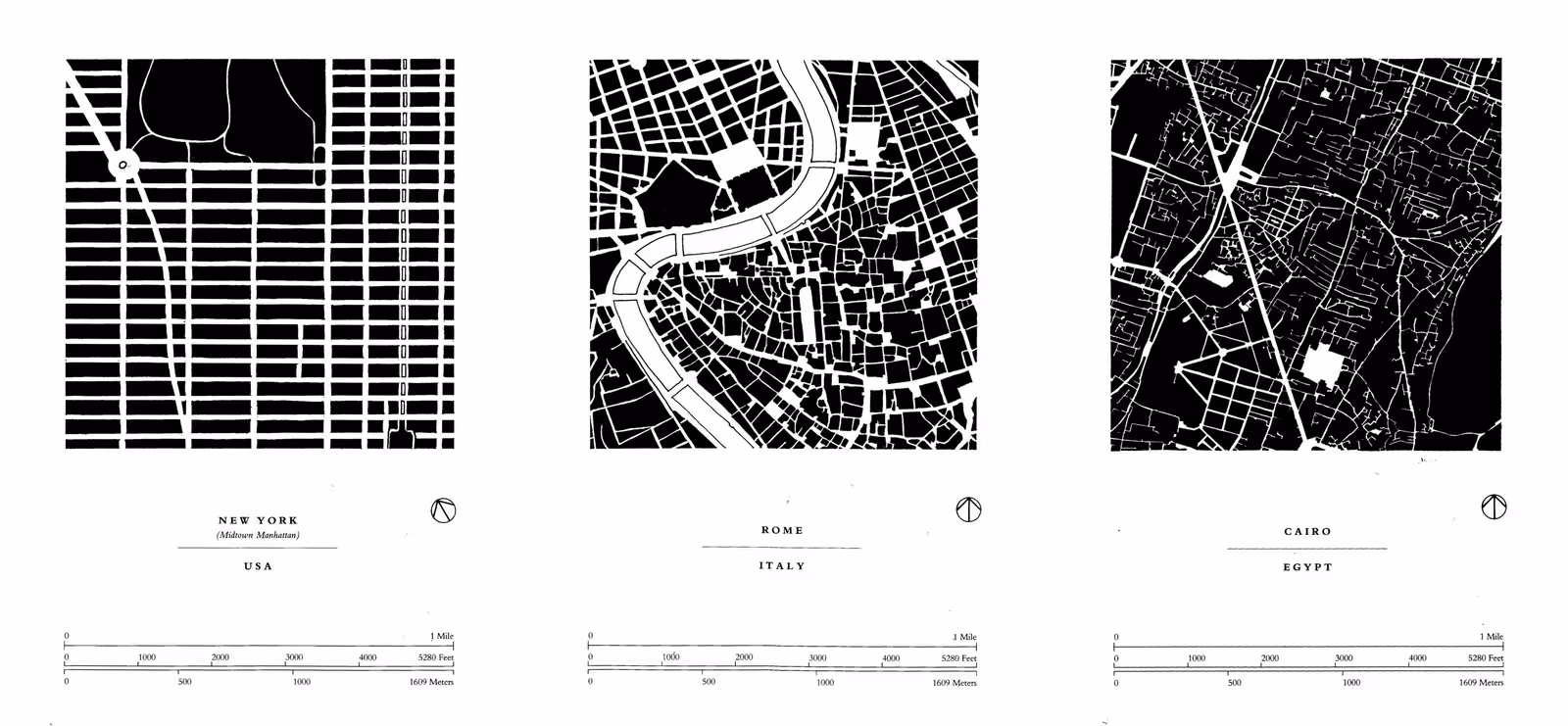
The figure above shows three city street networks with varying levels of permeability. An area with higher intersection density requires less out of direction travel to get from point A to point B, so distances are shorter and more conducive to taking trips without a car.
First, we import the necessary Python libraries:
#| output: false
#| message: false

import osmnx as ox
import matplotlib.pyplot as plt
import geopandas as gpd
import seaborn as sns
import numpy as np
import pandas as pd
import pandana as pnda
# select city and crs
cityname = 'kuala lumpur, malaysia'
crs = 32647# obtain graph of the city
graph = ox.graph_from_place(cityname, network_type="walk")
# project graph onto our crs
graph = ox.projection.project_graph(graph, to_crs=crs)# simplify our graph to exclude non-intersections
graph_simplified = ox.simplification.consolidate_intersections(
graph,
tolerance=5, # buffer around each node (project the graph beforehand)
rebuild_graph=True,
dead_ends=False, # remove cul-de-sacs
reconnect_edges=True
)# obtain nodes and edges and pass it as gdfs
nodes, edges = ox.graph_to_gdfs(graph)
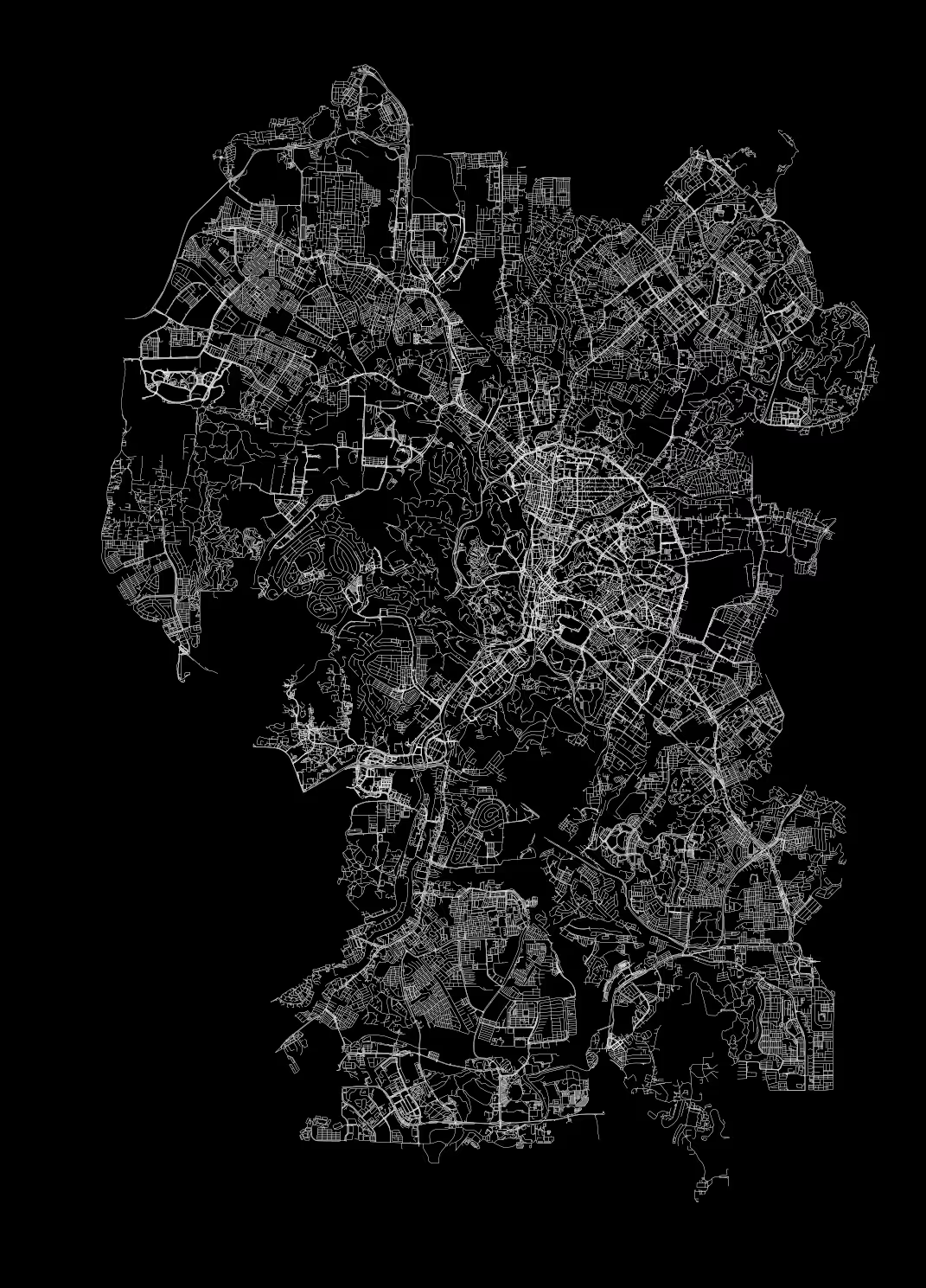
nodes_s, edges_s = ox.graph_to_gdfs(graph_simplified)@fig-graphkl depicts the graph representation of the street networks of Kuala Lumpur. At first glance, we observe that the street designs are closely adapted to its terrain. Unlike the gridiron plan of New York and Kyoto, Kuala Lumpur follows an organic layout that is responsive to its topography, leading to curvilinear streets and irregular lots. The extent of street network is also limited by some areas with forest reserves and/or hill fomrations.
#| label: fig-graphkl
#| fig-cap: "A graph representation of Kuala Lumpur"

# plot a base graph of the street network of kuala lumpur
fig, ax = plt.subplots(figsize=(20,15))
ax.set_aspect('equal')
ax.set_facecolor('black')
fig.set_facecolor('black')

edges.plot(
    ax=ax,
    color='white',
    linewidth=0.2
)

plt.tight_layout()

plt.savefig('/output/kl_graph.png')
A heatmap of intersection density
To obtain the intersection density of the city, we divide the entire street network into equally sized area. We then count up the number of intersection in each area. @fig-intrscthexmap shows the intersection per hexagonal area.
#| label: fig-intrscthexmap
#| fig-cap: "Intersection counts per hexbin"

# setting plot style parameters
COLOR = 'white'
plt.rcParams['text.color'] = COLOR
plt.rcParams['axes.labelcolor'] = COLOR
plt.rcParams['xtick.color'] = COLOR
plt.rcParams['ytick.color'] = COLOR

fig, ax = plt.subplots(figsize=(20,15))
ax.set_aspect('equal')
fig.set_facecolor('black')
ax.set_facecolor('black')

hb = ax.hexbin(
    x=nodes_s['x'],
    y=nodes_s['y'],
    gridsize=[75,65],
    cmap='viridis',
    mincnt=1,
    vmax=70,
)

cb = plt.colorbar(hb, ax=ax, shrink=0.4, ticks=[1, 20, 40, 60, 80, 100])
cb.ax.tick_params(color='none', labelsize=20)
cb.ax.set_yticklabels(['1', '20', '40', '60', '80', '>= 100'])
cb.set_label('Intersections per hexagon', fontsize=20, fontweight='bold')

plt.tight_layout()

plt.savefig('/output/intersection_hexbin.png')
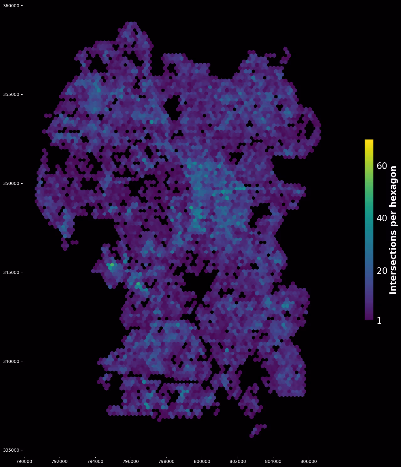
From @fig-intrscthexmap, we see that intersection-dense areas are concentrated around the Central Business District (CBD), surrounded by Jalan Tun Razak. This area include places such as Pasar Seni, Kampung Baru, Bukit Bintang and the like. Small disconnected spots of highly intersected areas can also be found in Bangsar-Universiti Malaya, and Kepong area.
The uneven intersection densities across the city mean that certain areas are not as permeable as others, making getting around in those areas more difficult by walking. Whereas accessing places in areas with higher permeability is easier by foot. Apart from that, moving from one place to the next in the same area is also easier by foot, further incentivising walking within these areas. It is no wonder why the CBD area is known for its tourism and dense office buildings.
import plotly.express as px
import plotly.subplots as sp
import plotly.io as pio
# get the binned data from the hexbin object
counts = hb.get_array()
verts = hb.get_offsets()

counts_unmasked = counts.filled(np.nan)
int_counts = np.array([round(i) for i in counts_unmasked])
#| label: fig-histhexbin
#| fig-cap: Histogram of intersection count hexbin distribution
pio.renderers.default = "notebook"
# plot histogram
intersection_dist = px.histogram(int_counts,
labels={"value": "intersections in each bin"})
intersection_dist.update_layout(showlegend=False)@fig-histhexbin shows the distribution of the number of intersections across all binned intersection (each observation is one bin attached to a value of intersection counts). As a whole, the city doesn't appear to be evenly permeable — a majority of unit areas found in the city street network contains zero to ten intersections. Each equally-sized area of the city has, on average, roughly 8.27 intersections.
int_counts.mean().round(3)8.269Accessibility
Knowing how permeable a city is might not tell us a great deal about walkability. The spatial distribution of places of interest (POIs) also plays an important role. It is crucial that the design of urban spaces can ensure that sociable places and key amenities like parks, libraries, shops, schools, and hospitals are within reach of walking distance. But what does this mean exactly?
Carlos Moreno popularised the “15-minute city” concept, an urban design goal that emphasises proximity. A short definition of the concept reads:
The 15-minute city represents an urban model in which the essential needs of residents are accessible on foot or by bicycle within a short perimeter in high-density areas.
[@moreno15MinuteCitySolution2024]
The model suggests that travel time contributes to urban walkability. People are more likely to walk if destinations are a stone throw away. When key amenities are strategically placed within 15-minute radii, people are more likely to walk. A study conducted by MIT researchers found strong correlation between the accessibility of amenities within a 15-minute walk from home and the usage of those amenities [@abbiasov15MinuteCityQuantified2022]. Simply by having places that are close to each other can improve visits to and usage of those places. A high variety of places that are close to each other incentivises people to walk in taking journeys and performing their daily activities.
Measuring walking time to destinations
Proximity is a function of network distance — the shortest path or the lowest cost-time to travel between two locations, considering the network's structure and constraints. By analysing the city's street as networks, we can measure how walkable to each POI is within the city.
Each street of a city is an edge in a graph. Walking at a constant speed, each street has a travel time based on its length, we give each edge a travel time as its weight. Then we can compute how long it takes to walk 5, 10, 15 minutes away from each node.
In a graph, we can calculate how much time is spent walking down each edge to reach a node and in reverse, find how far we can reach within a map from that node.
To find how much time it takes to walk to any nearest POI in a city, we can reverse the calculation, by calculating how far you can reach away from the POI. However, it would be difficult to approximate how far you can walk from any POI without a reference point on the network. We can take any intersection (nodes on our network) as reference.
As the POIs of our interest may not lie directly on the network (for example, the exact coordinate of a hospital can be a little far from the streets, even though it is walkable from the street), we can approximate their position on the network by proxying it to the nearest intersection to the POI.
Thus, we can find how many intersections can be reach within a defined time if we start from the POI (now proxied at an intersection), and we will have an approximatation of how walkable is it to the nearest POI within any area in the city.
# collect metro station points from osmnx

place = "Selangor"
stations = ox.features_from_place(place, tags = {'railway':['station']})
stations = stations[stations['name'].notnull()]
#| output: false
# ensure all geometries are points
stations["geometry"] = stations.geometry.centroid#| label: tbl-stations
#| tbl-cap: Collected centroids of train and metro stations in Greater KL
stations
#| label: fig-proxplot
#| fig-cap: "Heatmap of walking time to nearest POIs"
# plot the walking time to nearest POIs
fig, ax = plt.subplots(figsize=(12,15))
ax.set_axis_off()
ax.set_aspect('equal')
fig.set_facecolor((0,0,0))
# plot distance to nearest POI
sc = ax.scatter(
x=nodes['x'],
y=nodes['y'],
c=distances[1],
s=1,
cmap='viridis_r',
)
cb = fig.colorbar(sc, ax=ax, shrink=0.4, ticks=[0, 300, 600, 900])
cb.ax.tick_params(color='none', labelsize=20)
cb.ax.set_yticklabels(['0', '5', '10', '>= 15'])
cb.set_label('Walking time to nearest POI (minutes)', fontsize=20, fontweight='bold')
plt.tight_layout()
plt.savefig('/output/walk_access.png')
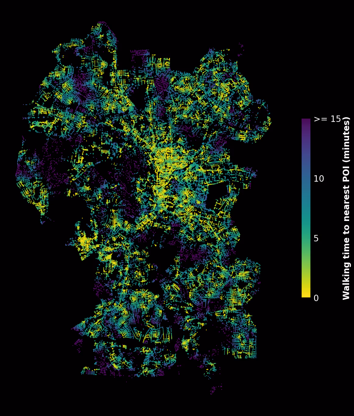
We collect the coordinates of amenity POIs like schools, hospitals, libraries, public services, townhalls, community centres, malls and parks throughout the city. We then look at the nearest 10 POIs from any POI.
@fig-proxplot shows the amount of time it takes to walk to the nearest ten POIs from any point on the street network. The brighter areas indicate that more POIs can be reached within shorter walking time. Being in the dimmer areas require 15 minutes or more to reach the nearest POI (in all directions). Brighter areas also signifies higher densities of POIs, making it easier to get from one to another in those areas.
Walkable POIs are distributed in patchwork throughout the city. Areas where walking to another POI takes more than 15 minutes are littered across and in between areas where the same walking takes shorter time. These darker patches could be geographically or topologically determined (e.g., forest reserves or river systems). Visually gauging the base graph ( @fig-graphkl ), we can conclude that this is the case generally.
Multi-modal connectivity
Walking is also complemented by other modes of transport. Most public transport journeys start and end with walk [@uitpWhyWalkingPublic2024]. Pedestrian-accessible public transport systems reduce the frequency of changing between modes, making journeys in the city frictionless.
To reduce car usage, sustainable public transport policies should promote pedestrian access to public transport. Currently, public transport connectivity outside the KL city centre is addressed by providing "Park-and-ride" option, allowing commuters to drive from nearby residential suburbs to Light Rail, Mass Rapid Transit or Land Commuter stations. This solution works to reduce the inbound vehicle traffic to city centre, but served to divert traffic elsewhere.
The solution only address the short-term problem of traffic management (and mostly inbound traffic). As more and more of the city outskirts develop into residential suburbs, and further into urban areas of their own right, traffic flow worsens in these areas, even creating problems of their own [@chanAuthoritiesUrgedAddress2025].
Direct foot access to public transport is key to increase public transport usage, this means making access to public transport points like metro and bus stations walkable. Like the exercise above, we can assess the walkability of public transport points by finding the walking time on the street networks towards each public transport point. To do this, we can rely on isochrones.
# collect metro station points from osmnx
place = "Selangor"
stations = ox.features_from_place(place, tags = {'railway':['station']})
stations = stations[stations['name'].notnull()]#| output: false
# ensure all geometries are points
stations["geometry"] = stations.geometry.centroid
#| label: tbl-stations
#| tbl-cap: Collected centroids of train and metro stations in Greater KL

stationsIsochrones visually represent the travel time to a point in a network. Isochrones are typically computed by generating shortest-path trees on graphs, then generating a convex hull around the accessible POI. Put differently, each concentric ring of the isochrone represent the further extent one can reach by walking within a fixed duration. The wider the isochrones, the further one can walk out of direction from that point within the same time, making it more accessible by walking. For example, taking five minutes to walk to a train station
We draw isochrones around a random sample of LRT, MRT and KTM stations in Greater Kuala Lumpur to produce the average out of direction travel distance, based on 5 minutes, 10 minutes and 15 minutes on foot, assuming the same walk speed. To do this, we use the openreouteservice API provided by HeiGIT. We visualise this in @fig-stationisochrones.
#| output: false
#| message: false

import folium
from shapely.geometry import shape

import os
import time
from dotenv import load_dotenv
import openrouteservice
from openrouteservice import client

load_dotenv()  # reads .env

ORS_API_KEY = os.getenv("ORS_API_KEY")
client = openrouteservice.Client(key=ORS_API_KEY)

# get the first station to initialize the map
first_station = stations.iloc[0]
center_lat, center_lon = first_station.geometry.y, first_station.geometry.x

# define a folium map
m = folium.Map(
    location=[center_lat, center_lon],
    zoom_start=13,
    tiles="cartodbpositron"
)

#| output: false

# iterate over all stations
walk_time = [300, 600, 900]
colors_map = [ "#2ca02c", "#1f76b4a0", "#ff7f0e",]  # example hex colors

for _, station in stations.sample(50).iterrows():
    lon, lat = station.geometry.x, station.geometry.y
    # plot isochrones using openrouteservice
    iso = client.isochrones(
        locations=[[lon, lat]],
        profile="foot-walking",
        range=walk_time,
    )

    iso_gdf = gpd.GeoDataFrame(
        [{"geometry": shape(f["geometry"]), "value": f["properties"]["value"]} for f in iso["features"]],
        crs="EPSG:4326"
    )
    # plot each isochrone with its corresponding color
    for val, color in zip(walk_time, colors_map):
        subset = iso_gdf[iso_gdf["value"] == val]
        folium.GeoJson(
            subset,
            style_function=lambda feature, c=color: {
                "fillColor": c,
                "color": c,
                "fillOpacity": 0.3,
                "weight": 1
            }
        ).add_to(m)

    folium.Marker([lat, lon], popup=station["name"]).add_to(m)

    time.sleep(2)  # avoid rate limit

#| label: fig-stationisochrones
#| fig-cap: Isochrones of walking time to random sample of stations by 5, 10 and 15 minutes

m
A birds-eye-view of walkability
Now that we have an idea of what walkability looks like in Greater KL using urban morphological measures, let's put together an index to compare across localities in Greater KL. We use the same measures of permeability based on overall intersection density, and accessibility based on POI proximity to derive a simple composite score of walkability. We compare walkability of localities of the Greater KL conurbation and create a harmonised index using this score.
@fig-walkabilityidx shows the ranking of localities by walkability.
def calculate_poi_accessibility(localities, tags):
    """
    Calculates reachable POIs within 10 mins walk.
    """
    WALK_TIME_MIN = 10
    MAX_DIST_SEC = WALK_TIME_MIN * 60
    all_walktime = []

    for locality in localities:
        try:
            # 1. Get Street Network and project it
            G = ox.graph_from_place(locality, network_type="walk")
            G_proj = ox.project_graph(G)
            nodes_proj, edges_proj = ox.graph_to_gdfs(G_proj)

            # 2. Get POIs and project to match G
            pois = ox.features_from_place(locality, tags=tags)
            if pois.empty:
                continue
            pois_proj = pois.to_crs(nodes_proj.crs)

            # 3. Add travel times
            # Note: add_edge_speeds expects unprojected usually,
            # or use G_proj but ensure 'length' is in meters.
            G_proj = ox.routing.add_edge_speeds(G_proj, fallback=4.5)
            G_proj = ox.routing.add_edge_travel_times(G_proj)
            nodes = ox.graph_to_gdfs(G_proj, edges=False)[['x', 'y']]
            edges = ox.graph_to_gdfs(G_proj, nodes=False).reset_index()[['u', 'v', 'travel_time']]

            print(edges['travel_time'].describe())

            # 4. Pandana Network
            network = pnda.Network(
                node_x=nodes['x'],
                node_y=nodes['y'],
                edge_from=edges['u'],
                edge_to=edges['v'],
                edge_weights=edges[['travel_time']]
            )

            # 5. Pre-calculate nearest nodes for POIs to avoid redundant lookups
            # We use the projected coordinates
            # Extract centroids from the pois' geometries
            centroids = pois_proj.centroid
            poi_nearest_nodes = ox.nearest_nodes(G_proj, X=centroids.x, Y=centroids.y)

            # Link POIs to the network
            network.set_pois(
                category='my_pois',
                maxdist=MAX_DIST_SEC,
                maxitems=300,
                x_col=centroids.x,
                y_col=centroids.y
            )

            # 6. Calculate reachability
            # This returns travel times to the Nth nearest POI
            reachable_pois_df = network.nearest_pois(
                distance=MAX_DIST_SEC,
                category='my_pois',
                num_pois=300
            )

            is_under_limit = reachable_pois_df < MAX_DIST_SEC
            node_counts = is_under_limit.sum(axis=1)
            poi_reachable_counts = pd.Series(poi_nearest_nodes).map(node_counts)

            poi_scores_df = pd.DataFrame({
                'locality': locality,
                'POI_ID': pois.index,
                'Reachable_POIs_Count': poi_reachable_counts.values - 1 # Subtract 1 for self-reachability
            })

            all_walktime.append(poi_scores_df)

        except Exception as e:
            print(f"Error in {locality}: {e}")

    return all_walktime
def get_intersection_density(localities):
    """
    Get intersection density stats from OSMnx for all localities.
    """
    all_intersection_stats = []

    for locality in localities:
        try:
            # get street network and project it
            G = ox.graph_from_place(locality, network_type="walk")
            G_proj = ox.project_graph(G)
            nodes_proj, edges_proj = ox.graph_to_gdfs(G_proj)

            # get geocode gdf for area calculation
            gdf = ox.geocode_to_gdf(locality)
            gdf_proj = ox.projection.project_gdf(gdf)

            area_m2 = gdf_proj.geometry.area.iloc[0]

            # get graph stats
            graph_stats = ox.basic_stats(G_proj, area = area_m2)
            intersection_stats = pd.DataFrame({
                'locality': [locality],
                'area_m2': [area_m2],
                'intersection_count' : [graph_stats['intersection_count']],
                'intersection_density_km' : [graph_stats['intersection_density_km']],
                'street_density_km' : [graph_stats['street_density_km']]
            })

            all_intersection_stats.append(intersection_stats)

        except Exception as e:
            print(f"Error in {locality}: {e}")
    return all_intersection_stats
gkl_localities = [
    "Kuala Lumpur, Malaysia",
    "Putrajaya, Malaysia",

    "Petaling Jaya, Selangor, Malaysia",
    "Shah Alam, Selangor, Malaysia",
    "Subang Jaya, Selangor, Malaysia",
    "Klang, Selangor, Malaysia",

    "Ampang Jaya, Selangor, Malaysia",
    "Kajang, Selangor, Malaysia",
    "Selayang, Selangor, Malaysia",
    "Rawang, Selangor, Malaysia",

    "Sepang, Selangor, Malaysia",
    "Kuala Langat, Selangor, Malaysia",
    "Kuala Selangor, Selangor, Malaysia"
    ]

# select points of interest based on osm tags
tags = {
    'amenity':['school',
               'college',
               'university',
               'library',
               'hospital',
               'public_service',
               'post_office',
               'townhall',
               'community_centre'],
    'shop':['mall'],
    'leisure':['park']
}
#| output: false
gkl_intersection_stats = get_intersection_density(gkl_localities)
Error in Rawang, Selangor, Malaysia: Found no graph nodes within the requested polygon.
#| label: tbl-intersectionstats
#| tbl-cap: Permeablity statistics by Greater KL locality

permeability_score = pd.concat(gkl_intersection_stats, ignore_index = True)
permeability_score
#| output: false
gkl_poi_accessibility = calculate_poi_accessibility(gkl_localities, tags)
count    200854.000000
mean          6.310265
std          12.933485
min           0.013223
25%           1.547974
50%           3.702406
75%           7.682236
max        1471.852000
Name: travel_time, dtype: float64
Generating contraction hierarchies with 8 threads.
Setting CH node vector of size 71818
Setting CH edge vector of size 200854
Range graph removed 205530 edges of 401708
. 10% . 20% . 30% . 40% . 50% . 60% . 70% . 80% . 90% . 100%
count    21012.000000
mean        21.877582
std         61.330871
min          0.028598
25%          2.697636
50%          6.613761
75%         16.201957
max       1677.562015
Name: travel_time, dtype: float64
Generating contraction hierarchies with 8 threads.
Setting CH node vector of size 7406
Setting CH edge vector of size 21012
Range graph removed 21828 edges of 42024
. 10% . 20% . 30% . 40% . 50% . 60% . 70% . 80% . 90% . 100%
 100% count    66284.000000
mean        12.097153
std         32.800624
min          0.012130
25%          2.348127
50%          5.106279
75%         10.583654
max       1166.291690
Name: travel_time, dtype: float64
Generating contraction hierarchies with 8 threads.
Setting CH node vector of size 23718
Setting CH edge vector of size 66284
Range graph removed 67782 edges of 132568
. 10% . 20% . 30% . 40% . 50% . 60% . 70% . 80% . 90% . 100%
count    128338.000000
mean         15.473566
std          49.150037
min           0.064617
25%           3.130550
50%           6.491836
75%          13.483481
max        3704.855416
Name: travel_time, dtype: float64
Generating contraction hierarchies with 8 threads.
Setting CH node vector of size 48432
Setting CH edge vector of size 128338
Range graph removed 132204 edges of 256676
. 10% . 20% . 30% . 40% . 50% . 60% . 70% . 80% . 90% . 100%
count    85738.000000
mean        10.949571
std         28.619641
min          0.064644
25%          2.920598
50%          5.776164
75%         10.222416
max       1122.127213
Name: travel_time, dtype: float64
Generating contraction hierarchies with 8 threads.
Setting CH node vector of size 30784
Setting CH edge vector of size 85738
Range graph removed 87702 edges of 171476
. 10% . 20% . 30% . 40% . 50% . 60% . 70% . 80% . 90% . 100%
 100% count    130252.000000
mean          9.338935
std          39.279349
min           0.031060
25%           2.441887
50%           4.423675
75%           8.288388
max        2398.546341
Name: travel_time, dtype: float64
Generating contraction hierarchies with 8 threads.
Setting CH node vector of size 49270
Setting CH edge vector of size 130252
Range graph removed 132396 edges of 260504
. 10% . 20% . 30% . 40% . 50% . 60% . 70% . 80% . 90% . 100%
#| label: tbl-accessibilitystats
#| tbl-cap: Accessibility statistics by Greater KL locality

gkl_poi_accessibility_c = pd.concat(gkl_poi_accessibility, ignore_index=True)
accessibility_score = gkl_poi_accessibility_c.groupby('locality')['Reachable_POIs_Count'].agg(
    mean_reach = 'mean',
    max_reach = 'max',
    min_reach = 'min',
    total_pois = 'count'
).reset_index()
accessibility_score
import scipy
from scipy.stats import zscore

walkability_score = pd.merge(permeability_score, accessibility_score, on = "locality")

def compute_walkability_index(df):
    """
    Calculate harmonized walkablity scores and index from permeability and accessibilty measure.
    """
    # we use log1p (log(1+x)) to avoid errors if total_pois is 0
    # this rewards a city for having 100 vs 10 POIs more than 1000 vs 910
    df['log_poi_variety'] = np.log1p(df['total_pois'])

    # z scaling (The Python 'scale()')
    # We standardize ALL three components so they contribute equally
    # ddof=0 matches R's default population standard deviation calculation
    df['z_intersection'] = zscore(df['intersection_density_km'], nan_policy='omit')
    df['z_reach'] = zscore(df['mean_reach'], nan_policy='omit')
    df['z_variety'] = zscore(df['log_poi_variety'], nan_policy='omit')

    # 3. Harmonization with Weighting
    # Logic: 40% Connectivity, 40% Amenity Reach, 20% Total Variety
    df['walkability_index'] = (
        (df['z_intersection'] * 0.4) +
        (df['z_reach'] * 0.4) +
        (df['z_variety'] * 0.2)
    )

    # 4. Final 0-100 Score for Interpretation
    min_idx = df['walkability_index'].min()
    max_idx = df['walkability_index'].max()
    df['walkability_score'] = 100 * (df['walkability_index'] - min_idx) / (max_idx - min_idx)

    return df.sort_values(by='walkability_score', ascending=False)
# calculate harmonized measure of intersection density and mean number of pois accessible out of direction
#| label: tbl-walkabilityscore
#| tbl-cap: Normalised walkability scores and index based on permeablity and accessibility by Greater KL locality

walkability_index = compute_walkability_index(walkability_score)
walkability_index
#| label: fig-walkabilityidx
#| fig-cap: Harmonised index of permeability and accessibility

pio.renderers.default = "notebook"

# plot the index
walkablity_plot = px.scatter(walkability_index, x="walkability_index", y="locality")

walkablity_plot
What remains unseen: Quality of walk
The morphological measures are only able to capture the abstract, morphological features of walkability. They can tell the network distance of a place and the theoretical time it takes to walk there navigating the city streets. They remain limited by their assumptions about street networks and make no statements on how humans actually interact with pedestrian environments.
In reality, what makes people walk in the city is influenced by a myriad of factors. It is not only important to ask what makes walking easy, but also what makes walking enjoyable? These are subjective factors of walking often related to the immediate experience of walking in the city, and not captured by morphological measures like permeability or accessibility.
Safety and comfort are two key street attributes that influence subjective walkability [@loukaitou-siderisItSafeWalk12006]. Safety and comfort are sometimes attributes of the physical environment: a steep walk up a hill, potholes and existence of continuous paved walkways can affect people's preference of walking. The design of built environments like dedicated pedestrian paths, the width of these paths, separation of travel modes sharing the same space, the existence of shield from weather elements, et cetera, all contribute to the walkability of an urban space.
Streetscapes are important: compare living streets along a park to major trunk roads filled with bustling automobiles. One is perceived to be more walkable than the other.
The perceptual and social elements are also important: vibrant neighborhoods with many other pedestrians are perceived to be safer, lined shopfronts also served as signifier of safety as people hang out around these spaces [@jacobsDeathLifeGreat1992].
It is beyond the length of this article to cover assessment methods of streetscapes and subjective walkability. However, it remains key that urban design account the subjective elements of walkability with the same importance as the "objective" forms of walkability.
Making streets that work for people
Urban spaces are political, no less its streets. The street is the primary urban public space that is shared among various actors: vehicles, people, road users, shop owners, et cetera. Hence, public spaces can be seen as a kind of commons — scarce resource that we must share among each other.
Like any commons, the use of this public space is contested. Optimising streets for cars require modifications or design decisions at the expense of other users, like pedestrians. For example, to accommodate car traffic, streets would have to expand multiple car lanes, raising speed limits and braking up connected footpaths. The same can be said about the effect of optimising streets for pedestrians on car mobility. The design of streets is also influenced by the built environment: the buildings that line streets constrain the available functional public space.
What sets streets apart from pastures as commons is that, the manner in which the commons is shared and distributed involves deliberate human interventions and decision-making.
Past mixture of automotive policy, urban planning and physical development policies were geared towards real estate development and financialization, as well as institutions that prop up car and private property ownership. In a way, we can see street networks as spaces that reflect its political economy. Their structures and morphology, besides from being shaped by physical limits, are also a function of institutional constraints such as property regimes and political priorities.
Making streets that work for people means reclaiming the social purpose of public spaces that streets represent. Urban mobility that rely on cars can exclude a sizeable share of the city-dwellers that have no means to drive, such as the elderly, children and the differently-abled. By making streets walkable, we also make urban mobility more equitable. Un-walkable streets are also less friendly to tourists and businesses by constraining the foot-access to diverse sociable places. Making streets
### References

::: {#refs}
:::